What does "frequency" mean in an image?

Question

I don't understand how frequencies are defined in images/photographs. As far as I understand it now, high frequencies are like sharp things in images, like edges or so, and low frequencies are kind of the opposite?

I also would like to understand the outcome of Discrete Fourier Transformations, like how to read them properly.

It would be cool if somebody could explain to me the following:

1. What are frequencies in pictures and how are they defined?

2. How do you read the outcome of a Discrete Fourier Transformation?

Answer 1

I will only answer the first question: What are frequencies in images?

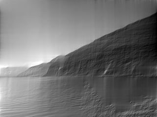
Fourier Transform is a mathematical technique where the same image information is represented not for each pixel separately but rather for each frequency. Think about it this way. The sea has waves some of which are very slow moving (like tides), others are medium in size and still some others are tiny like the ripples formed from a gust. You can think of them as three separate waves but at each point on the surface of the sea and a moment in time, you get just one height of water.

The same applies to images. You can think of the image being made up of various waves or frequencies. To create your image, start with the average colour (actually thinking of gray scale images is easier). Then add waves of different wave lengths and strength to slowly build up details in the picture.

Source Image:

First Frequency (Average):

The second frequency along the vertical dimension is a wave starting at zero at the bottom of the image, rising, becoming zero again along the centred horizon and falling below zero to finally become zero at the top of the image. (I described a Fourier Series without phase shift, but the analogy still holds.)

Here you can see the second frequency along the horizontal and vertical. Notice that you can make out where the mountain will be (dark) and where the sky and lake will be (lighter).

Second Frequency:

Each additional wave or frequency brings along more ripples and as such, more detail. To get different images, the wave height/amplitude can be changed as well as the starting point of the wave, also called the Phase.

Third Frequency:

Interestingly, the information amount is the same in this representation and one can go back and forth between normal images (spatial domain) and Fourier Transformed images (frequency domain). In the frequency domain we need to keep information of all frequencies along with the amplitude and the phase information.

Here it is using 50% of the frequencies:

There are variants of all this, with distinctions to be made among Fourier Series, Fourier Transform and Discrete Fourier Transform and Discrete Cosine Transform (DCT).

One interesting application is in the use of compression algorithms like JPEG. Here the DCT is used to save more of the important parts of the image (the low frequencies) and less of the high frequencies.

I wrote this in the hope that novice readers can get a basic understanding of the idea of Fourier Transforms. For that I made some simplifications that I hope the more advanced readers will forgive me.

Animated

Video generated by Thomas Devoogdt can be viewed at Vimeo.

---

Frequencies in Post-Processing

There are numerous methods that rely on frequencies for post processing, mostly because we never look at single pixels individually. Many algorithms work on frequency because it is more natural to think about them this way. But also because the Fourier Transform contains the same information we can express any mathematical operation (or post processing step) in the frequency and the spatial domains! Sometimes the pixel-wise description is better but often the frequency description is better. (Better primarily means faster in this context.)

One technique I would like to point for no particular reason except that it is artists working directly with frequencies and that is *frequency separation *. I am not going to describe it but you can see how it works on YouTube for both Photoshop and GIMP.

You create two layers one with the low frequencies and one with the high frequencies. For portraits you can do skin smoothing on the high frequencies without affecting the skin tones in the low frequencies.

Code

This is some code to generate the above examples. It can be run as a simple Python program.

from PIL import Image
from numpy.fft import rfft2, irfft2
import numpy as np

def save_dims(ft, low, high, name):
    ft2 = np.zeros_like(ft)
    # copy the frequencies from low to high but all others stay zero.
    ft2[low:high, low:high] = ft[low:high, low:high]
    save(ft2, name)

def save(ft, name):
    rft = irfft2(ft)
    img = Image.fromarray(rft)
    img = img.convert('L')
    img.save(name)

def main():
    # Convert input into grayscale and save.
    img = Image.open("input.jpg")
    img = img.convert('L')
    img.save('input_gray.png')
    # Do Fourier Transform on image.
    ft = rfft2(img)
    # Take only zeroth frequency and do Inverse FT and save.
    save_dims(ft, 0, 1, 'output_0.png')
    # Take first two frequencies in both directions.
    save_dims(ft, 0, 2, 'output_1.png')
    save_dims(ft, 0, 3, 'output_2.png')
    # Take first 50% of frequencies.
    x = min(ft.shape)
    save_dims(ft, 0, x/2, 'output_50p.png')

def generateGif():
    ''' Generates images to be later converted to a gif.
    This requires ImageMagick:
    convert -delay 100 -loop 0 output_*.png animation.gif
    '''
    # Requires images2gif from code.google.com/p/visvis/source/browse/vvmovie/images2gif.py 
    # from images2gif import writeGif

    img = Image.open('input.jpg')
    img = img.convert('L')
    # Resize image before any calculation.
    size = (640,480)
    img.thumbnail(size, Image.ANTIALIAS)
    ft = rfft2(img)

    images = []
    for x in range(0, max(ft.shape)):
        ft2 = np.zeros_like(ft)
        ft2[0:x, 0:x] = ft[0:x,0:x]
        rft = irfft2(ft2)
        img_out = Image.fromarray(rft).convert('L')
        fname = 'animation/output_%05d.jpg' %(x, )
        img_out.save(fname, quality=60, optimize=True)

    #writeGif('animation.gif', images, duration=0.2)


if __name__=='__main__':
    main()
    #generateGif()

Answer 2

I will try to explain with the simplest math terms possible. If you want to skip the math, jump to part II, if you want to get the short answer skip to Part III

Part I

Frequency of a signal means the number of occurrences of a repeating event per unit of time. So if the unit of time is seconds then frequency is measured with Herz: 1Hz = 1/s. So a signal with 100Hz, has a pattern that repeats 100 times per second.

The most basic signal (from the point of view of signal processing) is a sinus signal.

y(t) = sin(2πft)

where f is the frequency of this sinus signal, and t is time. If this signal was sound and f was around 50Hz, you will hear one very low bass tone. with a higher frequency like 15kHz it will be a higher tone.

Now to generalise the concept, the signal could be a spacial signal, instead of a temporal signal... as if you draw the sinus wave on a piece of paper, with an axis called x pointing to the right, and the y axis perpendicular to the x axis.

y(x) = sin(2πfx)

where f is the frequency of the signal, and x is the spacial variable. f here is not measured with 1/s anymore, but 1/(unit of space).

Fourier a French mathematician showed that you can generate any signal by adding a number of sine and cosine signals with different amplitudes and frequencies. That is called Fourier Analysis.

Using Fourier analysis it is possible to write any function y(x) as a sum of sine and cosine signals with different frequencies, so a function y(x) can be rewritten in terms of several functions related to frequency Y(f). One can say that y(x) = Some_Function( Y(f) ). or Y(f)=Reverse_of_Some_Function(y(x))

The Fourier Transformation is the function F that transform a signal from the x domain, to the frequency domain.

Y(f) = F( y(x) )

y(x) = F_inv(Y(f))

F is an analogue function, Discrete Fourier Transformation DFT is the numerical approximation of F. Fast Fourier Transformation FFT is a way to do DFT optimised for speed.

Ok...

Part II

Now computer images are composed of pixels, and every pixel have an intensity value for Red, Green, Blue aka RGB values. In grayscale images the intensity for R, G, B of any pixel are equal, R=G=B=I so we can talk about I for grayscale images.

The 800px X 100px grayscale picture below was generated using I(x) = sin(2πfx) where f = 1 repetition/800px = 0.00125 repetition/px

You can generate it yourself with Python3

from PIL import Image, ImageDraw
from math import sin, pi

img = Image.new('RGB', (800,100), color='black')
draw = ImageDraw.draw(img)

#cacluate the frequency
n = 10 #repetitions
f = n/img.width #

#iterate of the width pixels
for x in range(img.width):
 #calculate the intensity i in that pixel x
 y = sin(2*pi*f*x - pi/2) #this will generate values between -1 and +1, -pi/2 is to make sure that i starts with value 0 in the next line.
 i = (255+255*y)/2 #shifting and scaling y so that the values are between 0 and 255
 draw.line((i,0,i,img.height), fill=(int(i),int(i),int(i)))

img.show()

The 800px X 100px grayscale picture below was generated using I(x) = sin(2πfx) where f = 10repetitions/800px = 0.0125 repetitions/px

Now it is easy to see that this image has a horizontal frequency of 10. Let's increase the frequency by a factor of 10, so that n = 100. f = 100/800 = 1/8 = 0.125 repetitions/px:

As mentioned earlier, you can represent any signal (1D grayscale image) as a sum series of sine signals (1D grayscale sine images) with different frequencies. Using the same logic and method, we can generalise the concept to the different R, G, B components of the 2D image, and even the 3D image or even 2D images + time (2D video) or 3D images + time (3D video).

Part III

So a 1D grayscale image A has higher frequencies than another grayscale image B if A has "finer" details.

You can generalise that principle to colored 2D and even 3D images. The finer the "details" of an image are the higher the frequency content of that image is.

So a blue sky is low frequency in comparison with an image of a flower.

You can learn more about this by reading about Fourier Analysis, and about Digital Image Processing.

Answer 3

Briefly, frequency refers to the rate of change. More precisely, the frequency is the inverse of the period of the change—that is, the amount of time it takes to cycle from one brightness (or whatever) to a different brightness and back again. The faster then change (e.g. from light to dark), the higher the visual "frequency" required to represent that part of the image.

In other words, you can think of frequency in an image as the rate of change. Parts of the image that change rapidly from one color to another (e.g. sharp edges) contain high frequencies, and parts that change gradually (e.g. large surfaces with solid colors) contain only low frequencies.

When we talk about DCT and FFT and other similar transforms, we're usually doing them on a portion of an image (e.g. for JPEG compression, edge detection, and so on). It makes the most sense to talk about the transforms, then, in the context of a transform block of a given size.

Imagine, if you will, a 32 pixel x 32 pixel block of image data. (This number is arbitrary.) Suppose that the image is a simple gradient that is white on the left side, black in the middle, and white on right side. We would say that this signal has a period that is roughly one wavelength per 32 pixels of width, because it goes through a complete cycle from white to black to white again every 32 pixels.

We might arbitrarily call this frequency "1" — 1 cycle per 32 pixels, that is. I vaguely recall that this is commonly called θ in transform textbooks, or maybe θ/2, but I could be remembering wrong. Either way, we'll call it 1 for now, because this truly is arbitrary in an absolute sense; what matters is the relationship between frequencies in a relative sense. :-)

Suppose you have a second image that is white at one edge, then faded twice as quickly so that it went from white to black, to white, to black, and to white again at the other edge. We would then call that frequency "2" because it changes twice as often over the width of that 32 pixel block.

If we wanted to reproduce those simple images, we could literally say that every row consists of a signal with a frequency of 1 or 2, and you would know what the images look like. If the images went from black to 50% grey, you could do the same thing, but you'd have to say that they had a frequency of 1 or 2 at an intensity of 50%.

Real-world images, of course, aren't just a simple gradient. The image changes frequently and not periodically as you scan from left to right. However, within a small enough block (e.g. 8 pixels, 16 pixels) you can approximate that row of pixels as the sum of a series of signals, starting with the average of the pixel values in the row, followed by the amount of the "frequency 0.5" signal (black on one side, fading to white) to blend in (or with a negative amount, the amount of that signal to subtract), followed by the amount of frequency 1, frequency 2, frequency 4, and so on.

Now an image is unique in that it has frequency in both directions; it can get lighter and darker when moving both horizontally and vertically. For this reason, we use 2D DCT or FFT transforms instead of 1D. But the principle is still basically the same. You can precisely represent an 8x8 image with an 8x8 grid of similarly sized buckets.

Images are also more complex because of colors, but we'll ignore that for now, and assume that we're looking only at a single greyscale image as you might get by looking at the red channel of a photograph in isolation.

As for how to read the results of a transform, that depends on whether you're looking at a 1D transform or a 2D transform. For a 1D transform, you have a series of bins. The first is the average of all the input values. The second is the amount of the frequency 1 signal to add, the third is the amount of the frequency 2 signal to add, etc.

For a 2D transform, you have an n x n grid of values. The upper left is typically that average, and as you go in the horizontal direction, each bucket contains the amount of signal to mix in with a horizontal frequency of 1, 2, 4, etc. and as you go in the vertical direction, it is the amount of signal to mix in with a vertical frequency of 1, 2, 4, etc.

That is, of course, the complete story if you're talking about a DCT; by contrast, each bin for an FFT contains real and imaginary parts. The FFT is still based on the same basic idea (sort of), except that the way the frequencies are mapped onto bins is different and the math is hairier. :-)

Of course, the most common reason to generate these sorts of transforms is to then go one step further and throw some of the data away. For example, the DCT is used in JPEG compression. By reading the values in a zig-zag pattern starting with the upper left (the average) and moving towards the lower right, the most important data (the average and low-frequency information) gets recorded first, followed by progressively higher frequency data. At some point, you basically say "this is good enough" and throw away the highest-frequency data. This essentially smooths the image by throwing away its fine detail, but still gives you approximately the correct image.

And IIRC, FFTs are also sometimes used for edge detection, where you throw away all but the high frequency components as a means of detecting the areas of high contrast at sharp edges.

National Instruments has a nice article that explains this with pictures. :-)

Answer 4

Imagine scanning the image line by line with a photocell, and feeding the results to a plotter (these flat machines that make black waves on paper), oscilloscope (these boxes that make flickery green waves on a screen) or spectrum analyzer(bigger boxes that make green or multi colored picket fences). Or a loudspeaker even. The finer the structures in an image, the higher the frequencies (the pitch in the loudspeaker) of the signal shown/heard will be. The more contrast there is in the fine structures, the higher the amplitude of the high-frequency parts of the signal will be.